
|
Boletín de la Sociedad Geológica Mexicana Volumen 70, núm. 3, 2018, p. 731- 760 http://dx.doi.org/10.18268/BSGM2018v70n3a8
|
 |
Titan2F code for lahar hazard assessment: derivation, validation and verification
Gustavo A. Córdoba1*, Michael F. Sheridan2, Bruce Pitman3
1Department of Civil Engineering, University of Nariño, Pasto, 52001, Colombia.
2Center for Geohazards Studies and Department. of Geology, University of Buffalo, Buffalo, NY 14260, USA.
3Center for Geohazards Studies and Department of Mathematics, University of Buffalo, Buffalo, NY 14260, USA
This email address is being protected from spambots. You need JavaScript enabled to view it.
Abstract
Debris flows, lahars, avalanches, landslides, and other geophysical mass flows can contain material in the order of O(106–1010) m3 or more. These flows commonly consist of a mixture of soil and rocks with a significant quantity of interstitial fluid. They can be tens of meters deep, and their runouts can extend many kilometers. The complicated rheology of such a mixture challenges every constitutive model that can reasonably be applied: The range of length and timescales involved in such mass flows challenge the computational capabilities of existing models. This paper extends recent efforts to develop a depth averaged “thin layer” model for geophysical mass flows that contain a mixture of solid material and fluid. Concepts from the engineering community are integrated with phenomenological findings in geoscience, resulting in a theory that accounts for the principal solid and fluid forces as well as interactions between the phases, across a wide range of solid volume fractions. A principal contribution here is to present drag and phase interaction terms that conform with the literature in geosciences. The Titan2F program predicts the evolution of the volumetric concentration of solids and dynamic pressure. The theory is validated with data from one-dimensional dam break solutions and with data from artificial channel experiments.
Keywords: Lahar, modeling, depth averaging, two phase flow, debris flow, dynamic pressure.
Resumen
Los flujos de escombros, lahares, avalanchas, deslizamientos y otros flujos de masa geofísicos, pueden contener material del orden de O(106–1010) m3 o más. Estos flujos consisten comúnmente en una mezcla de sólidos y rocas, con una cantidad significativa de fluido intersticial. Pueden tener decenas de metros de espesor y un alcance de muchos kilómetros. La reología complicada de esta mezcla desafía cualquier modelo constitutivo que pueda ser aplicado con solidez. El rango de longitudes y escalas de tiempo involucrados en estos flujos de masa desafía también las capacidades computacionales de los modelos existentes. Este trabajo extiende esfuerzos recientes para desarrollar modelos de “capas delgadas”, integrados en profundidad, para flujos de masa que contienen una mezcla de material sólido y fluido. Se integran conceptos ingenieriles con hallazgos fenomenológicos en las geociencias, que resultan en una teoría que tiene en cuenta las principales fuerzas de partículas y fluidos, así como las interacciones entre las fases a través de un amplio rango de fracciones volumétricas de sólidos. La principal contribución aquí, es presentar términos para el arrastre y la interacción entre fases, los cuales concuerdan con la literatura de las geociencias. El programa Titan2F predice la evolución de la concentración y presión dinámica. La teoría es validada con datos de soluciones unidimensionales para ruptura de presas y verificada con datos de experimentos de canales artificiales.
Palabras Clave: Lahar, Modelado, Profundidad promedio, Flujo de dos fases, Flujo de escombros, Presión dinámica, Verificación del modelo, Validación del modelo.
1. Introduction
Among debris flows, the most devastating phenomena are volcanic flows known as lahars. The name comes from Indonesia and describes flows whose solid phase mostly consist of material of volcanic origin (Tilling, 1996). Lahars are regarded as the second largest destructive volcanic hazard (Baxter, 1983; Blong, 1984; Tilling, 1989). During the past century, tens of thousands of people have been killed by volcanic flows and hundreds of thousands forced from their homes (Tilling, 1996; National Research Council, 1991; 1994). These two-phase mass flows containing water and solid particles are common in volcanic regions. They can be initiated by several mechanisms. For example, a volcanic explosion can be accompanied by large plumes and pyroclastic flows consisting of rock and gas that race along the surface of the mountain at speeds as high as 100 m/s (Sheridan, 1979). The hot ash can melt snow, creating a muddy mixture that knocks down trees and entrains rocks and boulders into the flow. Cotopaxi volcano in Ecuador is an example of a volcano that has produced many large lahars by this process (Pistolesi et al., 2013). Crater lakes on volcanoes can be another source of lahars; a recent example is the 2007 lahar of Ruapehu in New Zealand (Procter et al., 2010). An additional mechanism for initiating lahars is intense rainfall on hillsides that are devoid of vegetation with material like clay soils or volcanic ash exposed. An example of this type of lahar is the 1998 mudflow at Casita Volcano in Nicaragua that occurred during Hurricane Mitch and caused hundreds of deaths (Sheridan et al., 1999). Lahars can carry constituent particles that typically range from clay to boulder size and can propagate tens of kilometers before coming to rest (Procter et al., 2010). As the solid particle component becomes deposited, the resulting deposits can be up to 100 m thick (Legros, 2002). However, the typical deposits left after a debris flow passes are on the scale of meters.
Models that assume one phase, like pure fluid (Chow, 1969) or pure frictional models (Savage and Hutter, 1989), cannot represent the complex behavior of these kinds of flows (Iverson et al., 2010; Iverson, 2014). In order to develop a complete mathematical model of debris flows, two principal challenges must be overcome: rheology and scale. First, relations among granular material must be developed to describe granular material including clays, sands, pebbles and rocks, with interstitial water. Second, a computational method must be developed that extends over six orders of magnitude, as clay diameters are of the order of O(10-6) m and boulders are O(1) m. Neither of these challenges can be fully met at this time. This paper tries to strike a balance between fidelity to the physics of mass flows and computational feasibility. We describe a modeling effort that draws on innovation from engineering and geoscience, which postulate constitutive theory and fluid-solid interaction effects, and, through a depth averaging process, results in a system of equations that is computationally tractable.
The modeling effort here has its origins in the pioneering work of Savage and Hutter (1989). They began with mass and momentum balance laws based on a Coulomb constitutive description of dry granular material. By scaling and depth averaging, they developed a “thin layer” model for granular flows down inclines. Flow over general topography was addressed in Gray et al. (1999), Patra et al. (2005), and Pudasaini and Hutter (2003). Comparison of thin-layer model results to historic flows was presented for example in Sheridan et al. (2005), Charbonnier and Gertisser (2009) and Sulpizio et al. (2010). In Hutter et al. (2005), the appropriateness of these thin layer models was considered for several different types of geophysical flows. Much of the modeling effort in this direction was summarized in Pudasaini and Hutter (2007).
Iverson (1997) and Iverson and Denlinger (2001) argued that the presence of interstitial fluid fundamentally alters the behavior of geophysical flows, and fluid effects should be included in the constitutive behavior of the flowing material. Starting with equations of mixture theory (Bedford and Drumheller, 1983) and through a careful examination of experiments, past studies developed a system of mass and momentum balance laws for the mixture. Unfortunately, in this development a balance equation for the motion of pore fluid was not readily available. Instead, based on experimental data, a transport equation for the fluid was postulated.
A different approach, based on a fully three-dimensional model of two-phase flows, can be found in Dartevelle (2004) and Meruane et al. (2010) and. Another approach to modeling mud flows employs visco-plastic constitutive assumptions (Coussot, 1997; Balmforth and Craster, 1999; Mei et al., 2001; Ancey, 2007). The choice of a visco-plastic flow model drives the subsequent derivation, as well as the parameter fitting necessary for the constitutive relationship. The process of depth averaging a visco-plastic flow is always difficult. The interface between yielding and non-yielding material is itself a free surface that must be determined. This attribute requires the use of multiple layers in the model system, with all the resulting complexity.
Pitman and Le (2005) developed a two-phase thin-layer model of fluid and granular material. They begin with a fully three-dimensional model of two-phase flows, based on model equations in engineering (Jackson, 2000). The model equations are scaled and depth averaged. The resulting system of equations is not complete, and closure assumptions are required. With these assumptions, the mathematical system is shown to be hyperbolic under common conditions, and thus well posed (Pelanti et al., 2008). The model of Pitman and Le (2005) includes a drag term, which is the only term describing the interaction of the two phases; this coefficient must then be fitted to experiments. That model assumes the fluid is not viscous, and that there is no frictional dissipation in the fluid phase at the basal surface. Both of these assumptions, which are reasonable in bench-scale fluidized bed experiments, are difficult to determine for large mass flows. The Pitman and Le (2005) model over-simplifies the physics of the fluid phase. When applied to real-scale topographies it only works for constant solid-particle concentrations well above the dilute flow limit, where the physics of two phase flows are mainly governed by pure fluid dynamics. Particle-particle interactions are unimportant for volumetric particle concentrations less than 10% (Bagnold, 1962; Winterwerp, 1999; Dartevelle, 2003). In order to address some of the shortcomings of the Pitman and Le (2005) model, this paper reconsiders the model equations proposed by them and proposes a revision of the model equations that better represents two-phase geophysical flows. For example, the proposed model accounts for the friction at the wall of the fluid phase and no longer assumes a constant volumetric fraction of solids, as in Valentine and Wohletz (1989) and Dobran (1991).
2. Model derivation
The Titan2F model uses a similar framework to that developed in Pitman and Le (2005). However, a complete set of model equations for a granular phase and for a fluid phase is written. Phase interaction terms are modeled, and scaling of all terms suggests simplifications that can be made. Depth averaging and closure assumptions complete the derivation.
A note on sign convention: in soil mechanics it is common to consider compressive stresses as positive; by contrast, in fluid mechanics, as an increase in pressure results in a reduction of the volume, compression is negative. We caution the reader to observe the sign convention in the equations below.
2.1 Fundamental assumptions
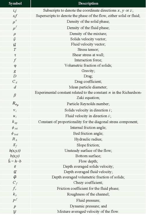
All symbols used in this paper are described in Table 1, Appendix A. The fundamental theory of two-phase flows used here can be found in Dobran (1991) and Jackson (2000). In two-space dimensions we consider a thin layer of granular material (s) and interstitial fluid (f), each of constant specific density ps and pf, respectively, flowing over a smooth basal surface, b. Erosion and deposition are neglected. Along the basal surface, we define a Cartesian coordinate system Oxyz, with origin O defined so the Oxy is tangent to the basal surface, with x in the downstream direction, and Oz in the normal direction. Writing  ,
,  for the velocities of the solid and fluid constituents, respectively, φ for the solid volume fraction and φf for the fluid volume fraction. We assume the mass is fully saturated, so the sum of the solid and fluid volume fractions adds to one (φf = 1 − φ). When writing equations in component form, we use subscripts to denote the component of the vectors, and superscripts the phase of the flow (either solids or fluid).
Mass conservation for the two constituent phases may be written as in Anderson and Jackson (1967):
|
|
|
(1) |
|
|
 |
(2) |
The momentum equations are:
|
|
|
(3) |
|
|
 |
(4) |

Here Ts and Tf are the stress tensors for the solid and fluid, respectively, and fs and ff are the interaction forces between the solid and fluid phases, respectively. We must postulate constitutive relations and an equation for the interphase force to close the system. Jackson (2000) presented an argument for separating buoyancy from other interphase force terms (such as drag or virtual mass), and for properly accounting for buoyancy in a field with fluid pressure variations. Similar modeling can be found in Valentine and Wohletz (1989), Dobran et al. (1993), Dobran (2001), and Neri et al. (2003, 2007).
Pitman and Le (2005) accounted only for the drag in evaluating the interaction force, unlike them, from Dobran (1991), (neglecting capillarity, virtual mass, and lift) we account for the total fluid stress as well:
|
|
|
(5) |
|
|
|
|
Here, the total fluid stress is ![]() f, where Pf is the fluid pressure and τf is the viscous contribution to the fluid stress. The drag term exchanges momentum between the phases, with a coefficient D that is phenomenological. Ergun (1952), Wallis (1969), Gidaspow (1994), Fan and Zhu (1998), Dobran (2001), Mazzei and Lettieri (2007) and Panneerselvan et al. (2007), among other sources, suggested values. When φ → 0, the drag vanishes. Following Mazzei and Lettieri (2007), we set
f, where Pf is the fluid pressure and τf is the viscous contribution to the fluid stress. The drag term exchanges momentum between the phases, with a coefficient D that is phenomenological. Ergun (1952), Wallis (1969), Gidaspow (1994), Fan and Zhu (1998), Dobran (2001), Mazzei and Lettieri (2007) and Panneerselvan et al. (2007), among other sources, suggested values. When φ → 0, the drag vanishes. Following Mazzei and Lettieri (2007), we set
|
|
|
(6) |
where d is the mean particle diameter and β is a constant related to the constant n in the Richardson–Zaki equation (Khan and Richardson, 1989). According to Mazzei and Lettieri (2007), this constant equals 2.80 either when ![]() or
or ![]() , thus we use β = 2.80 in Equation 6. Finally, by assuming smooth spherical particles on the inertial regime, the drag coefficient is approached as constant Cd = 1, which holds for particle Reynolds number up to 500 (Sparks et al., 1997).
, thus we use β = 2.80 in Equation 6. Finally, by assuming smooth spherical particles on the inertial regime, the drag coefficient is approached as constant Cd = 1, which holds for particle Reynolds number up to 500 (Sparks et al., 1997).
2.2 Scaling
The characteristic thickness of the flowing granular material is H and the characteristic length is L. We scale x and y by L, and z by H, the time by the free fall time ![]() . And we scale the x, y and z velocities by
. And we scale the x, y and z velocities by ![]() and
and ![]() , respectively. The stresses are scaled by psgH for the solids phase and pfgH for the fluid phase. After scaling, the mass balance equations are unchanged. Several terms in the momentum equations contain the factor ε = H/L, which is small; values of ε from 0.01 to 0.001 are not uncommon (Iverson and Denlinger, 2001). Writing x, y, z for x1,x2,x3, the solid momentum balance equations become (showing here just the x momentum),
, respectively. The stresses are scaled by psgH for the solids phase and pfgH for the fluid phase. After scaling, the mass balance equations are unchanged. Several terms in the momentum equations contain the factor ε = H/L, which is small; values of ε from 0.01 to 0.001 are not uncommon (Iverson and Denlinger, 2001). Writing x, y, z for x1,x2,x3, the solid momentum balance equations become (showing here just the x momentum),
|
|
= |
(7) |
Note that components of gravity have been scaled by the magnitude |g|, so (gx, gy, gz) is a unit vector.
With the same scaling, the fluid momentum balance equations become
|
|
 |
(8) |
Equation 8 shows an important advance in modeling the physics of the flow related to Pitman and Le (2005) as we do not neglect the effect of the volumetric fraction of fluids.
In summary, the proposed equation system consists of the solid volume fraction φ, the three solid velocities ![]() , and three fluid velocities
, and three fluid velocities ![]() . These variables evolve according to the six momentum balance laws for the species, and the mass conservation relations for each species.
. These variables evolve according to the six momentum balance laws for the species, and the mass conservation relations for each species.
2.3 Constitutive assumptions and boundary conditions
The upper surface of the flowing mass at Fh(x,y,t) = 0 is assumed to be a material surface and stress free. At the base of the mass, material is assumed to flow tangent to the basal surface, and to satisfy a sliding friction law. For the solid constituent, this friction relation specifies that the shear traction and the normal stress are proportional: ![]() , where
, where ![]() is the basal friction angle and the −sgn(v) specifies that the shear traction opposes motion.
is the basal friction angle and the −sgn(v) specifies that the shear traction opposes motion.
We now will discuss constitutive relations. A Coulomb constitutive relation (Coulomb, 1776) is postulated for the material. The Coulomb law is a nonlinear relation among the components of Ts, and stipulated that material deforms when the total stress reaches yield, which means ![]() , where dev(Ts) = Ts− ½ tr (Ts)I is the stress deviator, tr (Ts) is the trace of the stress (the sum of the diagonal components), I is the identity tensor, and κ is a material parameter, and that as deformation occurs, the stress and strain-rate tensors are aligned. That is, the alignment condition specifies dev(Ts) = λ dev(V), where the strain-rate V = −1/2 (∇ῡ+∇ῡ) and tr denotes the transpose. To avoid a switching between plastic and non-plastic behavior, we assume the solid material is everywhere in plastic yield.
, where dev(Ts) = Ts− ½ tr (Ts)I is the stress deviator, tr (Ts) is the trace of the stress (the sum of the diagonal components), I is the identity tensor, and κ is a material parameter, and that as deformation occurs, the stress and strain-rate tensors are aligned. That is, the alignment condition specifies dev(Ts) = λ dev(V), where the strain-rate V = −1/2 (∇ῡ+∇ῡ) and tr denotes the transpose. To avoid a switching between plastic and non-plastic behavior, we assume the solid material is everywhere in plastic yield.
The full Coulomb relations are too complex to be used here. Two simplifications are proposed. First, at the basal surface, the boundary condition ensures proportionality and alignment of the tangential and normal forces. We assume the same proportionality and alignment holds throughout the thin flowing layer of material. Written in components ij, this implies Tijs = νijTzzs, where the proportionality constant ν is a function of φbed. Second, following Rankine (1857) and Terzaghi (1936), an earth pressure relation is assumed for the diagonal stress components, νii = kap, or Txxs = kapTzzs, where
|
|
|
(9)
|
Here φint is the internal friction angle and the choice of the plus or minus sign depends on whether flow is locally contracting (the passive state, with ![]() , and the plus sign), or expanding (the active state, with
, and the plus sign), or expanding (the active state, with ![]() , and the minus sign).
, and the minus sign).
For the fluid, the stress terms in Equation 8 should be such that in case of ϕs → 0 the equations agree with the pure fluid depth-averaged equations.
For pure water, the shear stress at wall can be approached by (Chow, 1969)
![]()
where ![]() is the slope friction and
is the slope friction and ![]() is the hydraulic ratio. Note that for shallow-water problems, this assumption could be considered a rough approximation in case the shallow-water theory's condition is not met. There are several approaches for approximating both the slope friction and the shear stress at wall For example, Pan et al. (2006) use the empirical Manning approach, whereas Liu and Leendertse (1978) and Zhou and Stansby (1999) use the Chezy equation. Both the Manning and Chezy approaches pose numerical problems when h → 0. Thus we use the Darcy equation (Zhou, 1995; Xu, 2006):
is the hydraulic ratio. Note that for shallow-water problems, this assumption could be considered a rough approximation in case the shallow-water theory's condition is not met. There are several approaches for approximating both the slope friction and the shear stress at wall For example, Pan et al. (2006) use the empirical Manning approach, whereas Liu and Leendertse (1978) and Zhou and Stansby (1999) use the Chezy equation. Both the Manning and Chezy approaches pose numerical problems when h → 0. Thus we use the Darcy equation (Zhou, 1995; Xu, 2006):
![]()
where
|
|
|
(10)
|
is the Chezy coefficient. The friction coefficient depends on the Reynolds number and the roughness of the channel (ks).
3. Depth averaging
The final step in the derivation is a depth averaging of the mass and momentum balance equations. In this and the following sections we will use the same notation used by Savage and Hutter (1989). If h(x,y,t) is the unsteady surface of the flow and b(x,y) is the terrain surface, for some function f, we compute
![]()
Where h − b is the flow depth at a point (x,y) and time t. As the function f contains partial derivatives, repeated use of the Leibniz rule is made to interchange integration and differentiation, and boundary conditions are employed to evaluate terms at b and h. In addition, several approximations must be made during the depth averaging process. In what follows, we only briefly sketch the depth averaging process, noting as appropriate those places where approximations are made. Pitman and Le (2005) provided an estimation of the errors typically made by these assumptions.
The terms of order ε are assumed small and we hope to drop all such terms from the model. However Savage and Hutter (1989) argued that diagonal contributions to the solid stress must be retained. Because there is no preferential downslope direction in our applications, and the flow direction may change during a flow, we retain the stress terms in both the x and y directions, dropping only O(ε) terms in the z direction. See the discussion in Iverson and Denlinger (2001).
3.1 Mass balance equation
As ρs and ρf are constants, Equation 1 can be reduced to :
![]()
Which says that the volume-weighted mixture flow is divergence free. This equation is integrated from z = b to z = h:
|
|
(11) |
The upper free surface Fh = 0 is a material surface for the mixture. So, following Savage and Hutter (1989) and Pitman and Le (2005), at z = h(x,y,t),
|
|
(12)
|
At the basal surface Fb = 0, the flow is tangent to the fixed bed, and the bed is fixed in time. Thus, we can drop in Equation 12 the terms in ∂t, taking into account that at the surface z = b(x,y) (Pitman and Le, 2005):
|
|
(13) |
Like in Pitman and Le (2005), at this point, we have ignored sedimentation, entrainment, and infiltration of fluid into the bed.
Using Equation 13 and after algebraic manipulation, the depth averaged equation for the total mass of the solid and fluid can be written
|
|
(14) |
In writing this equation, the depth averaged velocities are
![]()
with a similar expression for the volume fraction of solids ![]() and the other velocity components, and as in Savage and Hutter (1989),
and the other velocity components, and as in Savage and Hutter (1989), ![]() .
.
An additional equation is needed to solve for φ. After depth averaging Equation 1, we arrive at the mass balance equations for the solid and fluid phases:
|
|
(15)
|
Where ![]() =
= ![]() and
and ![]() =
= ![]() . From the saturation condition
. From the saturation condition
|
|
(16) |
3.2 z momentum
Note that as ε → 0 in the fluid z momentum equation, the fluid tends to be hydrostatic:
|
|
(17) |
Depth averaging Equation 17:
|
|
(18)
|
In the same manner, for the solid z momentum we find the equation for an effective stress:
|
|
(19) |
Substituting Equation 17 in 18 and solving for ∂zTszz,
![]()
Thus the normal solid stress in the z direction at any height is equal to the reduced gravity times the volumetric fraction of solids.
In scaling these equations, the z velocities have been dropped. Of course neglecting motion in the z direction is a central component of a thin layer theory. Furthermore, any contribution to the z momentum from fluid shearing—terms such a Tfxz, Tfyz—are dropped due to scaling. Thus, only pressure contributions to the fluid stress are important, which is an assumption we will make below, albeit with a modification at the basal surface.
3.3 x and y momentum
The nonlinearity of these equations presents difficulties in formulating a depth averaged theory, and complicates the derivation, and in several places it is necessary to take the depth average of products of terms. When necessary, we approximate the required closure relation; for example, as ![]() (Savage and Hutter, 1989; Pitman and Le, 2005).
(Savage and Hutter, 1989; Pitman and Le, 2005).
Considering first the equation for the motion of the solid phase, the left-hand side of the solids x momentum Equation 7 can be written
![]()
Depth averaging and using boundary conditions, we find
|
|
(20)
|
Now the depth average of the right hand side of Equation 7 becomes:
|
|
(21)
|
In order to proceed, the following assumptions are made:
• This equation governs the motion of the solid phase and we assume the upper free surface for the mixture is a free surface for both of the individual phases.
• The drag term ![]() is highly nonlinear and a correct depth average is all but impossible to calculate. We postulate that experiments could fit an averaged phenomenological drag of a similar form. As seen in Equation 6, we assume a drag coefficient
is highly nonlinear and a correct depth average is all but impossible to calculate. We postulate that experiments could fit an averaged phenomenological drag of a similar form. As seen in Equation 6, we assume a drag coefficient ![]() . In addition, as the range of particle sizes of lahars is huge, at present, tracking all of the particles or even a representative sample of them, is intractable. Nevertheless, the lahar mean class size is about coarse sand (Pareschi, 1996), thus we use a typical mean particle diameter for lahars d = 1 mm (Schmid, 1981).
. In addition, as the range of particle sizes of lahars is huge, at present, tracking all of the particles or even a representative sample of them, is intractable. Nevertheless, the lahar mean class size is about coarse sand (Pareschi, 1996), thus we use a typical mean particle diameter for lahars d = 1 mm (Schmid, 1981).
• The earth pressure relation for the solid phase is employed. That is, the basal shear stresses are assumed to be proportional to the normal stress
![]()
Where i can be either x or y, and the velocity ratio enforces that friction opposes motion in the designated direction (Savage and Hutter, 1989; Patra et al., 2005). The α notation will provide a convenient shorthand that we use in other places. Likewise the diagonal stresses are taken to be proportional to the normal solid stress
![]()
Finally, following Iverson and Denlinger (2001), xy shear stresses are determined by a Coulomb relation
![]()
Where the sgn function ensures that friction opposes straining in the (x,y) plane.
• For the fluid phase, the basal shear stresses are assumed to be proportional to the square of the depth averaged velocities (Zhuo, 1995; Xu, 2006)
![]()
Where ![]() is the Chezy coefficient, which depends on the friction coefficient (see Equation 9). A physical approach for this coefficient is the Colebrook–White equation (Colebrook and White, 1937), which for rough channels can be approximated as
is the Chezy coefficient, which depends on the friction coefficient (see Equation 9). A physical approach for this coefficient is the Colebrook–White equation (Colebrook and White, 1937), which for rough channels can be approximated as
|
|
(22)
|
Where ![]() is the roughness of the channel and is the hydraulic radius, which for shallow-water problems can be approached as the depth of the flow (
is the roughness of the channel and is the hydraulic radius, which for shallow-water problems can be approached as the depth of the flow (![]() ). Equation 22 is logarithmic, thus large uncertainties in
). Equation 22 is logarithmic, thus large uncertainties in ![]() result only in small variations in
result only in small variations in ![]() (Swaffield and Bridge, 1983). In the Transport & Road Research Laboratory (1976) guide, values of
(Swaffield and Bridge, 1983). In the Transport & Road Research Laboratory (1976) guide, values of ![]() are proposed for different materials and channel types. From that guide, we choose
are proposed for different materials and channel types. From that guide, we choose ![]() mm for channels in volcanic environments (as Titan2F is open source software, the user can modify this value). Therefore, here
mm for channels in volcanic environments (as Titan2F is open source software, the user can modify this value). Therefore, here ![]() will depend on the flow depth ĥ,
will depend on the flow depth ĥ, ![]() , and the fluid velocity
, and the fluid velocity ![]() . Note that this is a physical approach for
. Note that this is a physical approach for ![]() , which does not depend on empirical approaches.
, which does not depend on empirical approaches.
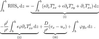
From Leibniz’s rule and the stress computations above, we find
|
|
(23)
|
Now using the fluid and solid stress relation
![]()
term (i) is approximated as
|
|
(24)
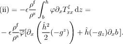
|
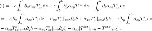
The upper free surface is stress free, so all terms involving ![]() vanish. The expression for (i) becomes
vanish. The expression for (i) becomes
|
|
(25)
|
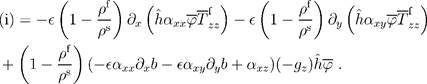
Note that the factor ![]() originates in the evaluation and depth averaging of the fluid stress; in typical flows, this factor is positive.
originates in the evaluation and depth averaging of the fluid stress; in typical flows, this factor is positive.
Combining all terms yields a solids x momentum equation
|
|
(26)
|
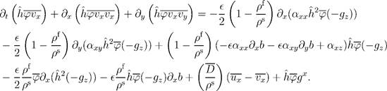
The y solid momentum equation can be derived in a similar fashion.
For pure fluids, the diagonal stresses and shear stress are zero. Thus, depth averaging the equation for the fluid motion presents fewer difficulties.
The depth averaged x momentum equation takes the form
|
|
(27)
|

Where ![]() Again, the fluid y momentum equation has a similar form. Note that unlike Pitman and Le (2005), if
Again, the fluid y momentum equation has a similar form. Note that unlike Pitman and Le (2005), if ![]() Equation 27 becomes the typical shallow-water approach of hydraulics (Chow, 1969). Kowalski (2008) describes how debris flows become reduced to a shallow-water flow as solid volume fraction vanishes.
Equation 27 becomes the typical shallow-water approach of hydraulics (Chow, 1969). Kowalski (2008) describes how debris flows become reduced to a shallow-water flow as solid volume fraction vanishes.
As noted above, we solve for volume fractions (φ), thus the bulk density can be calculated from
|
|
(28) |
Then, we obtain the dynamic pressure p from
|
|
(29) |
Where ![]() is the mixture averaged velocity of the flow (Fan and Zhu, 1998)
is the mixture averaged velocity of the flow (Fan and Zhu, 1998)
|
|
(30)
|
where ![]() and
and ![]() are the speeds of each phase.
are the speeds of each phase.
The use of the impacting dynamic pressure information on structures and living beings allows us to estimate levels of damage, as in Valentine (1998), Valentine et al. (2011), and Jones (2013), which is useful for vulnerability analysis.
4. Numerical solution
This system of equations (14, 15, 16, 26, 27) is then solved using the finite volume method, whose solution provides results of the velocity field, flow depth, and the volumetric concentration of solids at the center of each finite volume computational grid.
To solve the balance laws, we use the Godunov solver developed by Davis (1988) already implemented in Patra et al. (2005) and Pitman and Le (2005). The adaptive meshing is used as well, which allows us to have very fine grids where indicators show high gradients, and coarser grids where low gradients are detected. The time step is adjusted from the Courant condition (Courant et al., 1928). The complexity of the equation system results in typical time steps of the order of 10−4 s. As consequence of this small time step, Titan2F becomes a computationally expensive tool.
The numerical solution of the above set of equations presents strong numerical sensitivity to Digital Elevation Model (DEM) errors and the quality of those maps. The DEMscan have regions where elevations are not well defined; they can have crossed contour levels or even infinite holes (Dalbey et al., 2008; Wechsler, 2007). Abrupt terrain changes, both actual or DEM artifacts, cause computations of gradients and curvatures to become unstable. In order to avoid such numerical problems, patching and intelligent smoothing of the DEMs are needed.
Based on the hyperbolicity analysis done by Pitman and Le (2005), we try to ensure it , imposing a minimum![]() m, a maximum
m, a maximum ![]() corresponding to a maximum packing concentration of 0.65, and a minimum
corresponding to a maximum packing concentration of 0.65, and a minimum ![]() that ensured stability. This constraint makes the program stable if a smooth DEM is used.
that ensured stability. This constraint makes the program stable if a smooth DEM is used.
The needed initial conditions are the location of the pile of material, its geometry, the volumetric solid concentration, and initial velocity. There is no inflow condition implemented yet. Inflow hydrograph can be approached using several piles, each one with different initial depths. The bed and internal friction are set internally to the fixed values of ![]() = 40º and
= 40º and ![]() respectively. Those values correspond to the bed and internal friction of dry smooth spheres moving on the assumed bed roughness size
respectively. Those values correspond to the bed and internal friction of dry smooth spheres moving on the assumed bed roughness size ![]() (see Miller and Byne, 1996; Kirchner et al., 1990; Webb, 2004). Nevertheless, both of these parameters can affect
(see Miller and Byne, 1996; Kirchner et al., 1990; Webb, 2004). Nevertheless, both of these parameters can affect ![]() . The doted line in Figure 1 shows how
. The doted line in Figure 1 shows how ![]() changes with
changes with ![]() for any fixed value of
for any fixed value of ![]() (Note that Williams et al. (2008) shows that Titan2D results are not strongly affected by
(Note that Williams et al. (2008) shows that Titan2D results are not strongly affected by ![]() , see Equation 9 ).
, see Equation 9 ). ![]() is a function of
is a function of ![]() , which is directly related to
, which is directly related to ![]() , as shown by Kowalski (2008).
, as shown by Kowalski (2008).
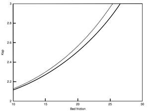
Figure 1. Effect on kap due to changes in φbed and j × φbed given a fix j. The black line shows the changes on kap related with φbed for any fixed j. The doted line shows the relation j × φbed with kap, used within the program.
The black line in Figure 1 shows how kap evolves when the fixed value of ![]() is multiplied by 0 < φ < 0.65. Thus, in the evaluation of
is multiplied by 0 < φ < 0.65. Thus, in the evaluation of ![]() we use the result of the multiplication
we use the result of the multiplication ![]() and
and
![]()
instead of the user defined ![]() and
and
![]()
used by Pitman and Le (2005). In this way, the range of resulting values of kap are within the ranges used for modeling lahars with Titan2D (Sheridan et al., 2005; Williams et al., 2008; Procter et al., 2010, 2012).
5. Differences with Pitman and Le model
There are six major differences between the present paper and Pitman and Le (2005):
1. In Pitman and Le (2005), mass and momentum conservation laws are derived for the solid material and for the phase averaged mixture of solid and fluid, whereas here, the Titan2F model uses mass and momentum equations for both individual phases.
2. Any two-phase model system must incorporate several phenomenological functions, such as an interphase drag coefficient. In the present derivation these functions are better adapted to geophysical flows whose fluid phase corresponds to water and the solid phase are rounded solid particles. The drag is calculated from an expression valid for the whole range of Reynolds numbers. It only needs the mean particle diameter of the flow as a parameter. We use a typical mean particle diameter of lahars. As Titan2F is open source, the user can modify the assumed value of the mean particle diameter.
3. The volumetric particle concentration is no longer a fixed parameter, which in our approach is calculated for every time step and grid point. This means that instead of having constant φ like in Equations (3.2) in Pitman and Le (2005) or simply not accounted for, like in the depth averaged fluid mass and momentum balance equations (3.27) and (3.28) in Pitman and Le (2005), we include the variable φ within all derivatives and depth averaged equations. Thus, in regions where the particle concentration vanishes, the solid phase role in the equation system vanishes as well. In that way, the equation system becomes the typical hydraulic shallow-water approach, which does not happen in Pitman and Le (2005).
4. We account for the fluid stresses at wall. We use a physical approach that only needs the roughness of the channel and the flow depth. The last term is calculated by the program at every time step, whereas the former is set as a fixed value.
5. The interaction forces between the phases now depend on both the drag and the fluid stress. The pressure is no longer the only term in the fluid stress model. Instead, we use the physical Darcy-Weisbach hydraulic approach that accounts for the full fluid stress. This approach allows us to have a more realistic model for the fluid phase than in Pitman and Le (2005).
6. The only input parameters needed by the program are the location of the pile of material, its volume, and the volumetric solids concentration. The friction coefficients are no longer needed as input as they are automatically adjusted according to the evolution of the volumetric fraction of solids across the grid and time. The bed and internal friction are set in such a way that when the volumetric fraction of solids tends to an assumed maximum packing concentration (φ = 0.65), both internal and bed frictions have a tendency to correspond to the values used in those cases in Titan2D. See Sheridan et al. (2005) and Williams et al. (2008) for ranges of values.
6. Validation and verification
Validation of the accuracy of the code was done with analytical solutions of the Dam Break problem and with several experimental results (e.g. Dressler, 1954; Ancey et al., 2008). Among them, we check the deposited pattern predicted by the program with the results shown by Liu (1996). The prediction of the arrival time and the flow-depth profile was compared with the experimental results shown by Iverson et al. (2010) from his recent work done on his large-channel facility.
Analytical solutions for shallow-water problems are scarce. Only one-dimensional analytical approaches are available in the literature, especially for the well known Dam Break problem (e.g., Dressler, 1954; Mangeney et al., 2000; Fernandez-Feira, 2006; Ancey et al., 2008). Unfortunately, analytical solutions for geo-mass flows are almost impossible to find due to the complexity of the nonlinear partial differential equations (Pudasaini and Hutter, 2007). Such solutions can be obtained only in special cases like the similarity based solutions proposed by Savage and Hutter (1989) for dry avalanches. In our test we use the solution proposed by Fernandez-Feira (2006) for the Dam Break problem on an incline for pure water. In our program we assume ![]() . Figure 2 shows a comparison of the Titan2F prediction with this analytical solution. The statistical t-test shows that there is no statistical difference between the analytical solutions and the prediction of Titan2F using the 1D version of the equations. That test shows that about 70% of the predictions of Titan2F can explain the analytical solution. At least for the one dimensional case, the program successfully reproduces analytical solutions for different initial conditions down to very low particle concentrations (less than 1%). However, as one dimensional approaches neglect lateral spreads, and at the initial parts of the flow evolution
. Figure 2 shows a comparison of the Titan2F prediction with this analytical solution. The statistical t-test shows that there is no statistical difference between the analytical solutions and the prediction of Titan2F using the 1D version of the equations. That test shows that about 70% of the predictions of Titan2F can explain the analytical solution. At least for the one dimensional case, the program successfully reproduces analytical solutions for different initial conditions down to very low particle concentrations (less than 1%). However, as one dimensional approaches neglect lateral spreads, and at the initial parts of the flow evolution ![]() is not small, that version of the program tends to over-estimate the front advance of the flow, as can be seen in Figure 2.
is not small, that version of the program tends to over-estimate the front advance of the flow, as can be seen in Figure 2.
Figure 2. Dam-break 1-D problem. Evolution of the flow-front depth with distance. The figure shows the result of the theoretical solution and the results from the numerical model for two initial conditions (1.5 m and 3 m). The statistical t-test shows that there is no statistically significant difference between the analytical solution and the predictions of Titan2F.
Liu (1996) performed several experiments for geo-mass flows in an inclined channel. He modified the initial volume, the channel slope, and the particle concentration to find the final size of the debris flows measured by their resulting maximum width and length. We reproduced the experimental final width and length after the simulation reached the same time corresponding to the duration reported by Liu (1996). Figure 3 shows the correspondence of the model with the experiments for (a) the width of the deposit and (b) the length. A Pearson correlation shows that 90% of the experimental data for the deposit length can be explained with the predictions of Titan2F, whereas 80% of the data for the deposit width can be explained by the predictions of the program. This illustrates the high accuracy of the program in predicting the deposit characteristics for different initial volumes (ranging from ![]() to
to ![]() ) and high initial solid concentrations (
) and high initial solid concentrations (![]() ). See Liu (1996) for details about initial conditions of his experiments.
). See Liu (1996) for details about initial conditions of his experiments.
Figure 3. Graphic comparison of the predictions of Titan2F with the experiments performed by Liu (1996). The results for several initial volumes compare (a) the width of the deposit and (b) the length of the deposit. The circles show data from the experiments, and the asterisks show the predictions of Titan2F.
The experiments performed by Iverson et al. (2010) done on a 95 m long artificial channel were used to verify the accuracy of the predictions of the flow front arrival time and the temporal evolution of the flow depth. These flows were unsteady and nonuniform. Iverson et al. (2010) show time-series data for several measured properties: flow thickness, pore pressure, basal normal stress, and arrival time of the front. Raw data provided to us was used to test the Titan2F prediction concerning time evolution of the flow depth and arrival times at the check points located at 32 and 66 m distance from the lock. As shown in Figures 4 and 5, the arrival time and the temporal evolution of the predicted depth fits well within the confidence interval of the experiments.
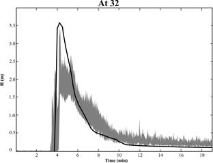
Figure 4. Verification of the accuracy of the Titan2F predictions for the time evolution of the flow depth and arrival of the front at 32 m distance from the lock. The black line represents the Titan2F results. The gray shadowed interval represents the confidence interval of the experiments performed by Iverson and co-workers (Iverson et al., 2010).
In both of the cases, Titan2F tends to over-estimate the flow depth just after the arrival of the front. This is probably an effect of the slight difference in the shape of the initial pile, as the free surface of the numerical pile follows the same slope of the channel, whereas the actual free surface within the lock is horizontal. Nevertheless, a Pearson correlation shows that more than 90% of this experimental data can be explained with the predictions of Titan2F.
Figure 5. Verification of the accuracy of the Titan2F predictions for the time evolution of the flow depth and arrival of the front at 66 m distance from the lock. The black line represents the Titan2F results. The gray shadowed interval represents the confidence interval of the experiments performed by Iverson et al. (2010).
The range of concentrations that the program can cope with are from ![]() (almost pure water) to
(almost pure water) to![]() (maximum packing concentration). Finally, as expected, the program predicts high particle concentrations at the front of the flow and low particle concentrations at the tail of the flow (in some cases, even near pure water concentrations, or φ → 0), as can be seen in Figure 6 where a longitudinal solids particle distribution predicted by Titan2F is shown. The predictions fit with the qualitative observation of Iverson et al. (2010) that the tail of the flow remains very watery.
(maximum packing concentration). Finally, as expected, the program predicts high particle concentrations at the front of the flow and low particle concentrations at the tail of the flow (in some cases, even near pure water concentrations, or φ → 0), as can be seen in Figure 6 where a longitudinal solids particle distribution predicted by Titan2F is shown. The predictions fit with the qualitative observation of Iverson et al. (2010) that the tail of the flow remains very watery.
Figure 6. Longitudinal distribution of the particle concentration (in %) after 14 s. The volumetric particle concentration at the upper part of the channel is very low, whereas at the end, the front of the flow becomes very concentrated, as noted by Iverson et al. (2010).
Using a predicted concentration of solids, the density is assessed (Equation 28), and, together with the speed of the flow, the dynamic pressure distribution is calculated as well (Equation 29). Despite that Iverson et al. (2010) do not show information about the dynamic pressure field, Titan2F does. Figure 7 shows a longitudinal section of the dynamic pressure after a 14 s simulation. Knowledge of the dynamic pressure information is of vital importance in risk analysis as structural damage and risk for human life can be assessed from it.
Figure 7. Longitudinal distribution of the predicted dynamic pressure at 14 s. The peak over-pressure occurs just at the end of the inclined part of the channel.
Verification with actual mud flows has been done as well, showing very good fit with field data. For example, Sheridan et al. (2011) shows that the Titan2F predictions are within 10% of the data shown by Procter et al. (2010) for the highly channeled mud flow at Ruapehu, New Zealand. In addition, the theory was tested against field data assessed by Williams et al. (2008) for the 2006 Vazcun creek lahar at Tungurahua volcano, Ecuador, as shown by Córdoba et al. (2015), where Titan2F predictions about maximum velocity are within 10% and within 15% for the measured super-elevation. In addition, Rodríguez-Espinosa et al. (2017) verified the accuracy of Titan2F predictions as well. They used the velocity measurements of the 2001 lahar in the Huiloac creek at Popocatapetl volcano, Mexico, done by Muñoz-Salinas et al. (2007), to compare Titan2F predictions. Using the non-parametric Kolmogorov (1933) confidence test, Rodríguez-Espinosa et al. (2017) show a significance level of 0.01.
7. Conclusions
We present a new computational two-phase tool for lahar hazard assessment that has no constraints on initial volumetric particle concentration other than the maximum packing concentration (![]() ). The program computes space–time evolution of the particle concentration, flow depth, velocity field, and dynamic pressure at each point of the computational grid.
). The program computes space–time evolution of the particle concentration, flow depth, velocity field, and dynamic pressure at each point of the computational grid.
The model is valid for two-phase flows whose phases consist of solids and water. However, the phenomenological approach used for the interphase drag model assumes an average diameter of the solids, which means individual boulders or particles cannot be tracked. In addition, the model is depth averaged, assuming thin layer and shallow-water approaches. Thus, our model correctly predicts the dynamics of gravity-driven flows providing the depth averaged values for the particle concentration, flow and phases velocities, and flow depth in a three dimensional topography. In order to model other kinds of geophysical mass flows, adjustments to the code must be done. For example, pyroclastic flows could be modeled if the flow density of the fluid phase is appropriately addressed (e.g., the effect of temperature on air density using ideal gas law and an additional equation for temperature).
The proposed mathematical approach allows for the simulation of a range of flow behaviors. Regions with almost pure fluid to regions of friction-dominated flows are correctly described by the equations. Using this information, dynamic pressure is deduced, which becomes a useful tool for risk assessment.
The highly nonlinear coupled-equation system makes the time step very small. The use of this new tool on natural terrains or detailed DEMs requires high computational power. The use of a high performance work station with multiple cores is advised.
Important processes that are not addressed by this tool include the effect of turbulence, incorporation of solid material from the bed of the channel, and incorporation of water into the flow from existing water bodies. Nevertheless, this two-phase flow is an important step forward in forming an acceptable computational model for simulating hazardous natural phenomena.
Acknowledgements
The authors wish to thank the economic support provided by the National Science Foundation Grant EAR 711497 aimed to the developing of Two-Phase-Titan. We also want to thank Ramona Stefanescu, Abani Patra, Dinesh Kumar, and Keith Dalbey from the University of Buffalo for the useful discussions about this development, and to Dr. Richard Iverson from the USGS who sent us the raw data of his experiments. The Universidad de Nariño, Colombia, provided supplementary support for this research. Esteban Mauricio Córdoba provided language help. Finally, we want to thank Sylvain Charbonnier and an anonymous reviewer for their useful reviews.
References
Ancey, C., 2007, Plasticity and geophysical flows: A review: Journal of Non-Newtonian FluidMechanics, 142, 4–35.
Ancey, C., Iverson, R.M., Rentschler, M., Denlinger, R.P., 2008, An exact solution for ideal dam-break floods on steep slopes: Water Resources Research, 44, W01430.
Anderson, T.B., Jackson, R., 1967, Fluid mechanical description of fluidized beds: Equations of motion: Industrial & Engineering Chemistry Fundamentals, 6, 527–539.
Balmforth, N.J., Craster, R.V., 1999, A consistent thin-layer theory for Bingham plastics: Journal of Non-Newtonian Fluid Mechanics, 84, 65–81.
Baxter, P.J., 1983, Health-Hazards of Volcanic-Eruptions: Journal of the Royal College of Physicians of London, 17, 180–182.
Bedford, A., Drumheller, D.S., 1983, Theories of immiscible and structured mixtures: International Journal of Engineering Science, 21, 863–960.
Blong, R.J., 1984, Volcanic Hazards: A Sourcebook on the Effects of Eruptions: Sydney, Australia, Academic Press Australia, 424 p.
Bagnold, R.A., 1962. Auto-suspension of transported sediment; turbidity currents. Proceedings of the Royal Society of London, Series A, Mathematical and Physical Sciences, 265, 315-319.
Charbonnier, S.J., Gertisser, R., 2009. Numerical simulations of block-and-ash flows using the Titan2D flow model: examples from the 2006 eruption of Merapi Volcano, Java, Indonesia, Bulletin of Volcanology, 71, 953-959.
Chow, V.T., 1959, Open channel hydraulics: New York, McGraw Hill, 680 p.
Colebrook, C.F., White, C.M., 1937, Experiments with fluid friction in roughened pipes: Proceedings of the Royal Society of London, Series A, Mathematical and Physical Sciences, 161, 367–381.
Córdoba, G., Villarosa, G., Sheridan, M.F., Viramonte, J.G., Beigt, D., Salmuni, G., 2015, Secondary lahar hazard assessment for Villa la Angostura, Argentina, using Two-Phase-Titan modelling code during 2011 Cordón Caulle eruption: Natural Hazards and Earth System Sciences, 15, 757–766.
Coulomb, C.A., 1776, Essai sur une application des regles de maximis et minimis a quelqes problemes de stratique, relatifs a l’architecture, in Memoires de mathematique & de physique, presentes a l'Academie Royale des Sciences par divers savans: Paris, De l'Imprimerie Royale, 343-382.
Courant, R., Friedrichs, K., Lewy, H., 1928, On the partial difference equations of mathematical physics: Mathematische Annalen, 100, 32–74.
Coussot, P., 1997, Mudflow rheology and dynamics: Rotterdam, A.A. Balkema, 272 p.
Pan, C. , Dai, S., Chen, S., 2006, Numerical simulation for 2D shallow water equations by using Godunov-type scheme with unstructured mesh: Journal of Hydrodynamics, 18, 475–480.
Dalbey, K., Patra, A.K., Pitman, E.B., Bursik, M.I., Sheridan, M.F., 2008, Input uncertainty propagation methods and hazard mapping of geophysical mass flows, Journal of Geophysical Research. 113, B05203, doi:10.1029/2006JB004471.
Dartevelle, S., 2003, Numerical and granulometric approaches to geophysical granular flows: Michigan, U.S.A., Michigan Technological University, Ph.D. Thesis, 132 p.
Dartevelle, S., 2004, Numerical modeling of geophysical granular flows: 1. A comprehensive approach to granular rheologies and geophysical multiphase flows: Geochemistry, Geophysics, Geosystems, 5, Q08003.
Davis, S.F., 1988, Simplified Second-Order Godunov-Type Methods: SIAM Journal on Scientific and Statistical Computing, 9, 445–473.
Dobran, F., 1991, Theory of Structured Multiphase Mixtures: Germany, Springer-Verlag, 225 p.
Dobran, F., 2001, Volcanic Processes: Mechanisms in Material Transport: New York, Springer, 590 p.
Dobran, F., Neri, A., Macedonio, G., 1993, Numerical simulation of collapsing volcanic columns: Journal of Geophysical Research, 98, 4231–4259.
Dressler, R., 1954, Comparison of theories and experiments for the hydraulic dam-break waves: International Association of Scientific Hydrology, 3(38), 319–329.
Ergun, S., 1952, Fluid flow through packed columns: Chemical Engineering Progress, 48, 89-94.
Fan, L., Zhu, C., 1998, Principles of Gas-Solid Flows: Cambridge, U.K., Cambridge University Press, 557 p.
Fernandez-Feira, R., 2006, Dam-break flow for arbitrary slopes of the bottom: Journal of Engineering Mathematics, 54, 319–331.
Gidaspow, D., 1994, Multiphase flow and fluidization: San Diego, U.S.A., Academic Press, 467 p.
Gray, J.M.N.T., Wieland, M., Hutter, K., 1999, Gravity-driven free surface flow of granular avalanches over complex basal topography: Proceedings of the Royal Society of London, Series A, Mathematical, Physical and Engineering Sciences, 455, 1841–1874.
Hutter, K., Wang, Y., Pudasaini, S.P., 2005, The Savage-Hutter avalanche model: How far can it be pushed?: Philosophical Transactions of the Royal Society of London A, Series A, Mathematical, Physical and Engineering Sciences, 363, 1507-1528.
Iverson, R.M., 1997, The physics of debris flows: Reviews of Geophysics, 35, 245–296.
Iverson, R.M., 2014, Debris flows: behaviour and hazard assessment: Geology Today, 30, 15–20.
Iverson, R.M., Denlinger, R.P., 2001, Flow of variably fluidized granular masses across three-dimensional terrain: 1. Coulomb mixture theory: Journal of Geophysical Research, 106, 537–552.
Iverson, R.M., Logan, M., LaHusen, R.G., Berti, M., 2010, The perfect debris flow? Aggregated results from 28 large-scale experiments: Journal of Geophysical Research, 115, F03005.
Jackson, R., 2000, The Dynamics of Fluidized Particles: Cambridge, U.K., Cambridge University Press, 343 p.
Jones, N., 2013, Damage of plates due to impact, dynamic pressure and explosive loads: Latin American Journal of Solids and Structures, 10, 767–780.
Khan, A.R., Richardson, J.F., 1989, Fluid-particle interactions and flow characteristics of fluidized beds and settling suspensions of spherical particles: Chemical Engineering Communications, 78, 111–130.
Kirchner, J.W., Dietrich, W.E., Iseya, F., Ikeda, H., 1990, The variability of critical shear stress, friction angle, and grain protrusion in water-worked sediments: Sedimentology, 37, 647-672.
Kolmogorov, A.N., 1933, Sulla determinazione empirica di una legge di distribuzione probabilita, Giornale dell'Istituto Italiano degli Attuari, 4, 1-11.
Kowalski, J., 2008, Two-Phase modeling of debris flows: Zurich, Switzerland, Eidgenossische Technische Hochschule (ETH), Ph.D. Thesis, 135 p.
Legros, F., 2002, The mobility of long-runout landslides: Engineering Geology, 63, 301–331.
Liu, S., Leendertse, J.J., 1978, Multidimensional numerical modeling of estuaries and coastal seas: Advances in Hydroscience, 11, 95–164.
Liu, X., 1996, Size of a debris flow deposition: model experiment approach: Environmental Geology, 28, 70–77.
Mangeney, A., Heinrich, P., Roche, R., 2000, Analytical solution for testing debris avalanche numerical models: Pure and Applied Geophysics, 157, 1081–1096.
Mazzei, L., Lettieri, P., 2007, A drag force closure for uniformly dispersed fluidized suspensions: Chemical Engineering Science, 62, 6129–6142.
Mei, C.C., Liu, K.-F., Yuhi, M., 2001, Mud Flow — Slow and Fast, in Balmforth, N.J., Provenzale, A. (eds.), Geomorphological Fluid Mechanics: Germany, Springer-Verlag Berlin Heidelberg, 548-577.
Meruane, C., Tamburrino, A., Roche, O., 2010, On the role of the ambient fluid on gravitational granular flow dynamics: Journal of Fluid Mechanics, 648, 381–404.
Miller, R.L., Byrne, R.J., 1966, The angle of repose for a single grain on a fixed rough bed: Sedimentology, 6, 303-314.
Muñoz-Salinas, E., Manea, V. C., Palacios, D., Castillo Rodríguez, M., 2007, Estimation of lahar flow velocity on Popocatépetl volcano (México): Geomorphology 92, 91–99.
National Research Council, 1991, The eruption of Nevado Del Ruiz Volcano Colombia, South America, November 13, 1985: Washington, D.C., U.S.A., The National Academies Press, 128 p.
Neri, A., Ongaro, T.E., Macedonio, G., Gidaspow, D., 2003, Multiparticle simulation of collapsing volcanic columns and pyroclastic flow: Journal of Geophysical Research, Solid Earth, 108, ECV 4-1Neri, A., Ongaro, T.E., Menconi, G., Vitturu, M., Cavazzoni, C., Erbacci, G., Baxter, P.J., 2007, 4D simulation of explosive eruption dynamics at Vesuvius: Geophysical Research Letters, 34, L04309.
Panneerselvan, R., Savithri, S., Surender, G.D., 2007, CFD based investigations on hydrodynamics and energy dissipation due to solid motion in liquid fluidised bed: Chemical Engineering Journal, 132, 159–171.
Pareschi, M.T., 1996. Physical modeling of eruptive phenomena: Lahars, in Scarpa, R., Tilling, R.I. (eds.), Monitoring and Mitigation of Volcano Hazards: Berlin, Germany, Springer-Verlag Berlin Heidelberg, 463-489.
Patra, A.K., Bauer, A.C., Nichita, C.C., Pitman, E.B., Sheridan, M.F., Bursik, M., Rupp, B., Webber, A., Stinton, A.J., Namikawa, L.M., Renschler, C.S., 2005, Parallel adaptive numerical simulation of dry avalanches over natural terrain: Journal of Volcanology and Geothermal Research, 139, 1–21.
Pelanti, M., Bouchut, F., Mangeney, A., 2008, A Roe-Type scheme for two-phase shallow granular flows over variable topography: ESAIM: Mathematical Modelling and Numerical Analysis, 42, 851–885.
Pistolesi, M., Cioni, R., Rosi, M., Cashman, K.V., Rossotti, A., Aguilera, E.., 2013, Evidence for lahar-triggering mechanisms in complex stratigraphic sequences: the post-twelfth century eruptive activity of Cotopaxi Volcano, Ecuador: Bulletin of Volcanology, 75, 698.
Pitman, E.B., Le, L., 2005, A two-fluid model for avalanche and debris flows: Philosophical Translations of the Royal Society of London, Series A, Mathematical, Physical & Engineering Sciences, 363, 1573–1601.
Procter, J.N., Cronin, S.J., Fuller, I.C., Sheridan, M., Neall, V.E., Keys, H., 2010, Lahar hazard assessment using Titan2D for an alluvial fan with rapidly changing geomorphology: Whangaehu River, Mt. Ruapehu: Geomorphology, 116, 162–174.
Procter, J.N., Cronin, S.J., Sheridan, M.F., 2012, Evaluation of Titan2D modelling forecast for the 2007 Crater Lake break-out lahar, Mt. Ruapehu, New Zealand: Geomorphology, 136, 95–105.
Pudasaini, S.P., Hutter, K., 2003, Rapid shear flows of dry granular masses down curved and twisted channels, Journal of Fluid Mechanics, 495, 193–208.
Pudasaini, S.P., Hutter, K., 2007, Avalanche Dynamics: Dynamics of Rapid Flow of Dense Granular Avalanches: Berlin, Germany, Springer-Verlag Berlin Heidelberg, 602 p.
Rankine, W.J.M., 1857, On the stability of loose earth: Philosophical Transactions of the Royal Society of London, 147, 9–27.
Rodríguez-Espinosa, D.M., Córdoba-Guerrero, G., Delgado-Granados, H., 2017, Evaluación probabilística del peligro por lahares en el flanco NE del volcán Popocatepetl, Boletín de la Sociedad Geológica Mexicana, 69, 243-260.
Savage, S.B., Hutter, K., 1989, The motion of a finite mass of granular material down a rough incline: Journal of Fluid Mechanics, 199, 177–215.
Schmid, R., 1981, Descriptive nomenclature and classification of pyroclastic deposits and fragments: Recommendations of the IUGS subcommision on systematics of igneous rocks: Geology, 9, 41–43.
Sheridan, M.F., 1979, Emplacement of pyroclastic flows: A review, in Chapin, C.E., Elston, W.E. (eds.), Ash-Flow Tuffs: U.S.A., Geological Society of America, 125–136.
Sheridan, M.F., Bonnard, C., Carreno, R., Siebe, C., Strauch, W., Navarro, M., Calero, J.C., Trujillo, N.B, 1999, Report on the 30 October 1998 Rockfall/avalanche and breakout flow of Casita Volcano, Nicaragua, triggered by hurricane Mitch. Landslide News, 12, 2-4.
Sheridan, M., Córdoba, G., Pitman, E., Cronin, S., Procter, J., 2011, Application of a wide-ranging two-phase debris flow model to the 2007 crater lake break-out lahar at Mt. Ruapehu, New Zealand (abstract), in American Geophysical Union Fall Meeting: San Francisco, California, U.S.A., American Geophysical Union, V53E-2691.
Sheridan, M.F., Stinton, A.J., Patra, A., Pitman, E.B., Bauer, A., Nichita, C.C., 2005, Evaluating Titan2D mass-flow model using the 1963 Little Tahoma Peak avalanches, Mount Rainier, Washington: Journal of Volcanology and Geothermal Research, 139, 89–102.
Sparks, R.S.J., Bursik, M.I., Carey, S.N., Gilbert, J.S., Glaze, L.S., Sigurdson, H., Woods, A.W., 1997, Volcanic Plumes: U.K., John Wiley and Sons, Inc, 557 p.
Sulpizio, R., Capra, L., Sarocchi, D., Saucedo, R., Gavilanes-Ruiz, J.C., Varley, N.R., 2010, Predicting the block-an-ash flow inundation areas at Volcán de Colima (Colima, Mexico) based on the present day (February 2010) status, Journal of Volcanology and Geothermal Research, 193, 49-66.
Swaffield, J.A., Bridge, S., 1983, Applicability of the Colebrook-White formula to represent frictional losses in partially filled unsteady pipeflow: Journal of Research of the National Bureau of Standards 88, 389–393.
Terzaghi, K., 1936, The shearing resistance of saturated soils and the angle between planes of shear: Proceedings of the First International Conference on Soil Mechanics and Foundation Engineering, 1, 54–56.
Tilling, R.I., 1989, Volcanic hazards and their mitigation: Progress and problems: Reviews of Geophysics, 27, 237–269.
Tilling, R.I., 1996, Volcanoes: U.S.A., U.S. Geological Survey, 45p.
Transport & Road Research Laboratory, 1976, A Guide for Engineers to the Design of Storm Sewer Systems: London, U.K., Department of the Environment, Road Note 35,30 p.
National Research Council, 1994, Mount Rainier: Active Cascade Volcano: Washington, D.C., USA, The National Academies Press, 128 p.
Valentine, G.A., 1998, Damage to structures by pyroclastic flows and surges, inferred from nuclear weapons effects: Journal of Volcanology and Geothermal Research, 87, 117–140.
Valentine, G.A., Wohletz, K.H., 1989, Numerical models of Plinian eruptions columns and pyroclastic flows: Journal of Geophysical Research, 94, 1867–1887.
Valentine, G.A., Doronzo, D.M., Dellino, P., Tullio, M., 2011, Effects of volcano profile on dilute pyroclastic density currents: Numerical simulations: Geology, 39, 947–950.
Wallis, G.B., 1969, One-dimensional two-phase flow: New York, U.S.A., McGraw.Hill, 408 p.
Webb, A., 2004, Granular flow experiments to validate numerical flow model, Titan2D: Buffalo, U.S.A., State University of New York at Buffalo, Department of Geology, Doctoral. Thesis, 130 pp. .
Wechsler, S.P., 2007, Uncertainties associated with digital elevation models for hydrologic applications: a review: Hydrology and Earth Sciences Discussions, European Geosciences Union, 11, 1481-1500.
Williams, R., Stinton, A.J., Sheridan, M.F., 2008, Evaluation of the Titan2D two-phase flow model using an actual event: Case study of the 2005 Vazcún Valley Lahar: Journal of Volcanology and Geothermal Research, 177, 760–766.
Winterwerp, J.C., 1999. On the dynamics of high concentrated mud suspension. Delft University of Technology, Faculty of Civil Engineering and Geosciences. Netherlads. Doctoral Thesis. 204 pp.
Xu, K., 2006, The gas-kinetic scheme for shallow water equations: Journal of Hydrodynamics, Ser. B, 18, 73–76.
Zhou, J.G., 1995, Velocity-depth coupling in shallow-water flows: Journal of Hydraulic Engineering, 121, 717–724.
Zhou, J.G., Stansby, P.K., 1999, 2D shallow water flow model for the hydraulic jump: International Journal for Numerical Methods in Fluids, 29, 375–387.
Appendix A
Table 1. Symbols used in this paper.
Manuscript received: February 20, 2017.
Corrected manuscript received: December 21, 2017.
Manuscript accepted: December 26, 2017.