
|
BOLETÍN DE LA SOCIEDAD GEOLÓGICA MEXICANA http://dx.doi.org/10.18268/BSGM2009v61n3a4 |
 |
3D velocity structure around the source area of the Armenia earthquake: 25 January 1999, Mw=6.2 (Colombia)
Velocidad estructural 3D alrededor del área fuente del sismo de Armenia del 25 de Enero de 1999, Mw=6.2 (Colombia)
Carlos Alberto Vargas–Jiménez1,*y Hugo Monsalve–Jaramillo2
1 Departamento de Geociencias. Grupo de Geofísica, Universidad Nacional de Colombia. Bogotá, Colombia.
2 Facultad de Ingeniería. Grupo Quimbaya, Universidad del Quindio. Armenia, Colombia.
* This email address is being protected from spambots. You need JavaScript enabled to view it..
Abstract
Selected P wave arrival time data of 518 events (mainly aftershocks) of the 25 January 1999 Armenia Earthquake (Mw=6.2, Colombia), recorded by 23 temporary seismic stations during February, 1999 to July, 2001, have been inverted simultaneously for both hypocenter locations and three–dimensional Vp structure. The surface geology of this area suggests a complex disposition of tectonic flakes composed by diverse rocks and crossed by the Romeral Fault System (RFS). However, there is a good correlation between high–velocity zones and old oceanic rocks affected by plutonic rocks. Metamorphic belts that wrap these rocks are well correlated with low–velocity zones. The disposition of tectonic flakes in depth is solved with a flower structure where the Cordoba fault slipped in a contact between high– and low–density rocks during the Armenia earthquake. The low–velocity zones would correspond to the older rocks that constitute the nucleus of the Central range. We infer that the source volume of the Armenia earthquake sequence lies within 75.64° – 75.72° W, 4.38° – 4.52°N and a depth of 5 – 21 km; the source volume is approximately 2 200 km3. Most of the well–located aftershocks occurred above the hypocenter of Armenia earthquake.
Key words: Local earthquake tomography, Armenia (Colombia), seismotectonic, Crust structure.
Resumen
Se seleccionaron tiempo de arribos de ondas P de 518 eventos (principalmente réplicas) del sismo de Armenia (Colombia) del 25 de enero de 1999 (Mw=6.2), registrados por una red temporal de 23 estaciones durante el período de Febrero de 1999 a Julio de 2001, han sido invertidas simultáneamente para localización de hipocentros y estructura 3D de velocidad de onda Vp. La geología superficial de esta área sugiere una compleja disposición de placas tectónicas compuesta por rocas diversas y atravesada por el sistema de fallas de Romeral (SFR). Sin embargo, haya una muy buena correlación entre zonas de velocidad alta y rocas oceánicas antiguas afectada por rocas plutónicas. Cinturones de rocas metamórficas que rodean estas rocas están bien correlacionados con zonas de baja velocidad. La estructura geológica en profundidad es resuelta con una estructura de flor donde la falla Córdoba se movió en el sismo de Armenia en un contacto entre rocas de alta y baja densidad. La zonas de baja velocidad corresponderían a rocas antiguas en la cordillera central. Inferimos que el volumen de la secuencia del sismo está entre las coordenadas 75.64°–75.72° W, 4.38°– 4.52° N y a una profundidad entre 5–21 km; el volumen es de 2 200 km3. La mayoría de las réplicas bien localizadas ocurrieron por encima del hipocentro del terremoto de Armenia.
Palabras Clave: Tomografía sísmica local, Armenia (Colombia), sismotectónica, estructura cortical.
1. Introduction
On 25 January 1999, at 18:19:16 UTC, an earthquake of magnitude M 6.2 took place in the central region of the Colombian Andes (Figure 1a). It claimed 1185 casualties, caused more than 4370 injured, and left about 160 000 people homeless. This earthquake was felt as far away as Cali, Medellin, and Bogotá where many high–rise buildings were shaken. The epicenter was located near Armenia city. This was one of the most important earthquakes occurred near an urban center in Colombia. Monsalve–Jaramillo and Vargas–Jimenez (2002) have located the epicenter at 75.669°W, 4.465°N, with a focal depth of 18.6 km, fault–plane solution  =8°, δ=65° and λ=–21°, and a stress drop of 28.4N/m2. Immediately after the main shock, the Instituto colombiano de geología y minería (INGEOMINAS) and the Observatorio Sismológico del Suroccidente de Colombia (OSSO) deployed temporary seismic stations to monitor the aftershocks. The Observatorio Sismológico de la Universidad del Quindío (OSQ) also installed five temporary stations in the area. Thus, a total of 23 temporary seismic stations were in operation to monitor the seismic activity for about 30 months; from February 1999 to July 2001. The hipocentral distribution of aftershocks has allowed to define a rupture area of about 124 km2 (Monsalve–Jaramillo and Vargas–Jimenez, 2002). The epicentral zone is dominated by a complex geology and has several active faults associated to the RFS. One branch of the RFS, locally named Cordoba fault, has been related to the main earthquake.
Because of the geotectonic context of central region of Colombian Andes, it has been scenario of several destructive events during the Twentieth Century (1938, Ms=7.0; 1961, Ms=6.7; 1962, Ms=6.7; 1979, Ms=6.7; 1995, Ms=6.6), the aftershocks can help us to know the crustal structure of the area. In fact, few studies have been carried out to investigate the seismic structure of this region. Ocola et al. (1975) first applied seismic high angle refraction studies from latitude 1°N to 4.5°N along the Eastern mountain Range. Their results revealed the Mohorӧvicic discontinuity about 52km deep. Meissner et al. (1976) did a high angle refraction throughout Colombo–Ecuatorian Trench around latitude 4°N. They found a subduction zone with the Mohorӧvicic discontinuity about 40km deep in the western sector of Colombia. Taboada et al. (2000) developed a seismotectonic study from stress analysis and proposed a scheme where overlapping of Caribbean over Nazca plates is responsible of differential angles of subduction and generates a Mohorӧvicic discontinuity deeper to north and east. Ojeda and Havskov (2001) inverted a 1D P– wave velocity (Vp) structure to the same region of this study. They reported a superficial Mohorӧvicic discontinuity about 32 km. Recently, a previous local earthquake tomography study using data from 1992 to 1999 and collected by Red Sísmica Nacional de Colombia (RSNC) exists, but it covers all the Andean region of Colombia and its scale shows regional Vp anomalies (Vargas et al, 2003). Their study area was focused on showing subduction structures associated to Nazca plate under the South America plate. They found low–velocity beneath volcanoes and high–velocity anomalies associated to old metamorphic belts that formed the East, Central, and Western mountain ranges. Two cross sections allowed suggesting different angles of subduction: in the southern region about 24° and in the northern region about 34°.
In this study we analyzed 518 events of the aftershocks collected by OSQ, about 3951 P–wave arrival time data, for simultaneous determination of the hypocentral parameters and estimation of P–wave velocity structure around the source area of the Armenia earthquake. Although it lacks the resolving power to constrain crustal anomalies, it provides us with structural reconstructions in the source area and its relation with seismotectonic of the RFS in this region.
2. Geological setting
The Colombian Andes constitutes a broad zone of continental deformation with a complex geological and tectonic configuration which is the result of the relative motions of three main plates: Nazca, South American and Caribbean (Figure 1a). Colombian Andes spreads into three ranges: Eastern, Central, and Western mountain ranges. The nature and composition of the Eastern, Central, and Western mountain ranges are substantially different; each one results from different tectonic processes that affected north–western South America. The RFS extends along the western boundary of the Central range and marks the limit between two lithologic domains: continental and oceanic towards the East and the West respectively (Mosquera, 1978; McCourt et al, 1984).
This region is composed of a pre–Mesozoic, polymetamorphic basement including oceanic and continental rocks such as Cajamarca complex (Figure 1b), covered by several volcanic sequences related to subduction (Barroso formation, Arquia complex, Quebradagrande complex, and Amaime formation). This basement is intruded by several Mesozoic and Cenozoic plutons (Igneous complex of Cordoba and Navarco river) that are covered by continental deposits and recent volcanic deposits (Penderisco, Cauca Superior, La Paila, Zarzal, and Glacis del Quindio formations). In general these rocks show a complex disposition of tectonic flakes affected by the RFS (Mosquera, 1978; McCourt et al, 1984; González y Núñez, 1991; Maya y González, 1995; Pardo y Moreno, 2001).
However, important seismic activity of Colombia is located along the RFS and follows distinct patterns, characterized by different depth ranges and tectonic regimes features. Detailed information of RFS in the Central Andean region is reported by Paris (1997) and Guzman et al. (1998). The most representative faults in the study area are: San Jeronimo, the most eastern fault of the RFS (Figure 1b); Córdoba and Navarco faults, associated with aftershocks distribution of the Armenia earthquake (Bohórquez et al, 1999); and the Armenia fault whose recent activity is evident in Armenia city. In general these faults are oriented NNE with almost vertical dips toward East and West. Its disposition in form of blocks is associated to a strike–slip system and presents left–lateral displacements. Monsalve–Jaramillo y Vargas–Jimenez (2002) reported that the distribution of aftershocks and focal mechanisms associate the Cordoba fault with the Armenia earthquake.
3. Analysis method and data
In the last decades seismology has increased the knowledge of the lateral heterogeneity in crustal structure for several regions of the world using three–dimensional inversion in function of local, regional, and teleseismic data (Aki and Lee, 1976; Crosson, 1976; Aki et al., 1977; Smith–son et al., 1977; Oliver, 1980; Zandt, 1981; Thurber, 1983; among others). Of course, with a frequency content comparable to seismic refraction signals, the local earthquake travel time data suit the purpose to illuminate the lateral variations of the velocity structure in the upper lithosphere much better. The inversion of –local earthquake travel time data follows approximately the method developed by Aki and Lee (1976) and Aki et al. (1977), with variations and adjustments, which are necessary because of the inherent differences in the input data and the forward and inverse problem. In contrast to the inversion of–teleseismic travel time data, the use of local earthquake data includes the problem of simultaneously, locating the earthquakes while inverting for a three–dimensional (3D) velocity field. This coupling of two inverse problems is the main reason for the different inversion procedure proposed for local earthquake data (Kissling, 1988). Many works have demonstrated the efficiency of this procedure, every time with more data and computational resources (Eberhart–Phillips et al., 1990; Eberhart–Phillips and Michael, 1993; Rietbrock, 1996; Eberhart–Phillips and Reyners, 1997; Thurber et al., 1997; Thurber and Kissling, 2000; Allen, 2001; Husen and Kissling, 2001; Kissling et al., 2001).
Because of active faults and seismotectonic areas can offer quality data to deduce crustal structures (Eberhart–Phillips and Michael, 1993; Eberhart–Phillips and Reyners, 1997; Chen et al., 2001), we performed an iterative, simultaneous inversion of hypocentral parameters and 3D –Vp structure in the source area of the Armenia earthquake using the SIMULPS13Q algorithm developed by Thurber (1983, 1993) and Eberhart–Phillips (1986, 1990). In SI–MULPS13Q– , travel times are computed using an approximate ray tracer with pseudo bending (Um and Thurber, 1987). After parameter separation, the inverse solution for Vp is obtained using a damped least squares technique; subsequently, hypocenters are relocated in the updated velocity model. Vp values were estimated at nodes of a 3D grid. By trial and error we found an adequate grid spacing of 5km with respect to reference point 75.42°W and 4.50°N (Figure 2). The nodes of the grid were spaced at depths 0.0 km, 5.0 km, 10.0 km, 15.0 km, 20.0 km and 30.0 km for a total of 1734 nodes. The depth 0.0 km coincides with the mean sea level.
3.1. Data and minimum 1D –Vp local model
Initially we selected 1337 local events recorded in the 23 stations with one–component 1 Hz L4–C seismometers. Five stations were equipped with telemetric data transmitters with digital system recording in SUDS format; three stations were equipped with MEQ–800 analog system and the rest digital system out of line. Arrival time was determined on the digital waveforms using an interactive processing software developed by the Observatorio Vulcanologico y Sismologico de Manizales (OVSM) and we read analogue waveforms over smoky paper. Phase weighting was applied based on estimated digital picking accuracy. We estimated an average digital picking accuracy of 0.1 s for P waves and 0.2 s for S wave, due that the digital system allows making zoom with this accuracy. These events were located with HYPO71 (Lee and Lahr, 1978) using the Ojeda and Haskov (2001) minimum 1D P–wave velocity (Vp) regional model. Their depuration allowed us to select 518 located events with a greater angle without observation as seen from epicenter (GAP) of <180°, RMS (Root mean square) values for the hypocenter locations < 0.3 s, and with at least 5 good P–observations. Because S–observations have high uncertainty and in most of the cases we did not recognize this phase, we did not estimate the S–wave velocity (Vs) structure.
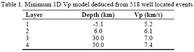
The 518 well located events with a total of 3 951 P–wave observations were selected to compute a minimum 1D –Vp local model for the source area of the Armenia earthquake using the program VELEST (Kissling et al., 1994; Kissling et al., 1995). Figure 2 shows the distribution of seismicity and its projection in depth that defines a rupture zone with dip toward East. Due to the dimensions of the recording array and the depth distribution of the earthquakes with almost no seismic activity below 25 km, the Moho is only poorly resolved by our data. Therefore, initial average crustal velocity was taken from the model obtained by Ojeda and Haskov (2001) for a large region of Colombia. We started the 1D inversion with a large number of thin layers (~1 km thick) and during the inversion process we combined those layers. The final layering of the minimum 1D model emerged from this process and reduced the data RMS residual by 87% from 1.53s to 0.20s (Table 1, Figure 3a). A series of tests to assess the quality of this 1D P–wave velocity model was then carried out. The inversion was started using initial models with average velocities significantly higher, lower, or randomly different than the minimum 1D P–model and with event location which were perturbed randomly in their three spatial coordinates. In general, the hypocenter locations are well recovered.
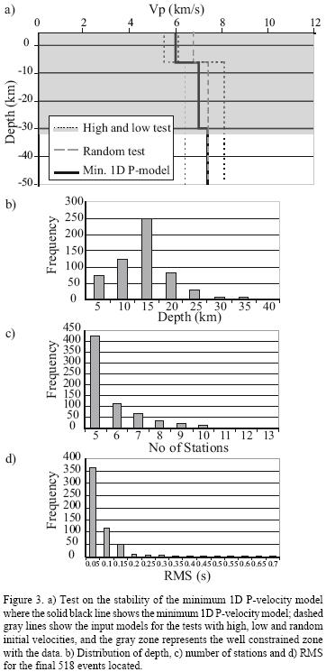
With regard to the velocity model, these tests show that from the top layer to 30 km depth, velocities are well constrained (gray zone in Figure 3a), but below 30 km the model is poorly constrained due to sparse sampling. On the other hand, we found a good correlation between station corrections and local geology under the seismological stations. In general, there are positive corrections in stations with young rocks and vice versa (Table 2). Figures 3b, 3c and 3d show the depth, number of stations, and RMS distribution of seismicity finally located with the minimum 1D P–model, where we see that the earthquake were located mainly between 10 to 20 km, which were recorded with more than 5 stations and their final solutions have RMS less than 0.2 s mainly.
3.2. 3D Tomography
A reliable interpretation of tomographic results requires an accurate analysis of the solution quality. Standard approaches comprise the use of synthetic tests such as checkerboard and geometrical anomalies associated with the characteristic model (Spakman and Nolet, 1988; Zhao et al., 1992; Zelt, 1998; Haslinger, 1999). We use a specifically designed synthetic model to estimate the capacity to restore the geometry and amplitude of the velocity structure. In our restoring resolution test we have used an uneven (low density) earthquake distribution with the true seismic array. The synthetic model was designed with two different laterally uniform velocity anomalies (thickness = 8 km)–over a semi–infinite medium (Figure 4a). Synthetic travel times were computed by a 3D elastic wave propagation routine based on finite differences (Cerjan et al., 1985; Nolet and Dahlen, 2000). Gaussian–distributed noise was added with a standard deviation range from 0.05 s. The synthetic data were inverted using the same parameterization and control parameters as for real data. Comparing the inversion results (Figure 4b) with the synthetic input model (Figure 4a) allows the identification of well–resolved areas in the central part of the model with resolution decreasing toward the outlying zone. The boundaries between high– and low–velocity anomalies were well resolved. In the deep layers there is not significant presence of velocity perturbations. This demostrates the capability of the parameterization, control parameters, and data set to resolve structures in the central part. Finally, the combination of the derivative weighted sum (DWS) and the resolution diagonal elements (RDE) are a good tool for describing the spatial ray sampling in the vicinity of a grid node and its independence with respect to the solution (Husen et al., 2000). Because the RDE depends strongly on the damping values, it was chosen based on a series of tests on the trade–off between model variance (roughness) and data variance (Eberhart–Phillips, 1986). Figures 4c and 4d display the RDE and DWS distributions of the inversion for the synthetic model. This information becomes more homogeneous in the central part of the model, thus confirming the good resolution estimated for the central regions
4. Results and discussion
Starting with a RMS for all events of 0.20s by the minimum 1D Vp–model, it was reduced to 0.12s by the 3D Vp–model (25%). Average values for location errors in the north–south, east–west and vertical directions were 0.73, 0.89, and 1.20 km respectively. In general, our sections show that it is not easy to have a direct interpretation of velocity anomalies (Figure 5). However, the scale of the surface geological structures in the study area (Figure 1b) is of the order of our grid–spacing and smaller. The tomographic results therefore represent a somewhat averaged (or low–pass filtered) image of the crustal velocities. Nevertheless some significant features can be recognized and compared with surface features. In the layer 0.0 km we see an area of high–velocity zones toward the central part with trend NNE. At depths 5.0 km, 10.0 km, 15.0 km, and 20.0 km this area has migrated toward SE and involved the hypocentral zone of the Armenia earthquake (see ellipse suggested in the figure 5). Surface geology of this area suggests a complex disposition of tectonic flakes composed by diverse rocks and crossed by the RFS. In this structural scenario we see a good correlation between high–velocity zones and old oceanic rocks (JKia, Kica and Kicq) affected by plutonic rocks (Kstd). The metamorphic rocks (Pzcc) that wrap these rocks are well correlated with low–velocity zones.
Figure 6 shows the Bouguer anomaly map of the study area (IGAC and INGEOMINAS, 1998) where we see high–density anomalies located toward the central part with trend NNE and wrapping low–density anomalies. This pattern coincides with velocity anomalies and oceanic rocks distribution. On the other hand, the Figure 7 shows three cross sections located at latitudes 4.4°N, 4.5°N and 4.6°N, where we see lower resolution toward–north the Armenia earthquake. The two more representative cross sections located at latitudes 4.4°N and 4.5°N allowed us to detect high–velocity zones that are interrupted by low–velocity zones in a horizontal and vertical pattern. In particular, a structural interpretation of the cross section at latitude 4.4°N (Figure 8) has been done following the structural model proposed by Ospina and Gallego (2002). In this interpretation we suggest that the disposition of tectonic flakes in depth be solved with a flower structure (Ospina and Gallego, 2002) where the Cordoba fault slipped in a contact between high–and low–density rocks during the Armenia earthquake. The low–velocity zones would correspond to the oldest rocks that constitute the nucleus of the Central mountain range such as Pzcc. Finally, because there is not significant change in the final hypocenter locations, we infer that the source volume of the Armenia Earthquake sequence lies within 75.64° – 75.72° W, 4.38° – 4.52°N and at a depth 5 – 21 km; the source volume is approximately 2.200 km3. Most of the well–located aftershocks occurred above the hypocenter of the Armenia earthquake (Figure 8).
Although there is a good correlation between the superficial observations, the 3D Vp inversion and the structural interpretation, it will be necessary to confirm this model with new geophysical evidences such as high–angle seismic profiles and detailed gravimetric surveys.
Acknowledgements
We are grateful to Lina Espinosa for her help to prepare the row data. Lina Ospina and Aracelly Gallego who worked hard and provided us with useful geologic data. We also thank Marisol Gomez for her important work to maintain the seismological network of OSQ. We are grateful to the OVSM and in general to INGEOMINAS for the technical support and helpful suggestions. This work was supported by the Centro de Investigaciones de la Facultad de Ingeniería of the Universidad del Quindio and the Geophysics Research Team at Universidad Nacional de Colombia, Sede Bogotá.
References
Aki, K. and Lee, W. H. K., 1976. Determination of Three–dimensional Anomalies under a Seismic Array Using First P Arrival Times from Local Earthquakes, 1. A Homogeneous Initial Model, J. Geophys. Res. 81 ,4381 – 4399.
Aki, K., Christoffersson, A., and Husebye, E. S., 1977. Determination of the 3–dimensional Seismic Structure of the Lithosphere, J. Geophys. Res. 82, 277–296.
Allen, R. M., 2001. The Mantle Plume beneath Iceland and its Interaction with the North–Atlantic Ridge: A Seismological Investigation, Ph.D. Thesis, Princeton University, 184 pp.
Bohórquez, O. P., Gil, F., Paiño, J., Monsalve, H., Osorios, J. A., Ospina, L. M., Acevedo, A. P. and Saenz, L., 1999. Estudio de réplicas asociadas al sismo del Quindio – Enero 25 de 1999. Rev. Sismol. Reg. Eje Caf., 4: 23–29.
Cerjan, C., Kosloff, D., Kosloff, R. and Reshef, M., 1985. A non–reflecting boundary condition for discrete acoustic and elastic wave equations, Geophysics, 50: 705–708.
Chen, C., Wang, W. and Teng, T., 2001. 3D Velocity Structure around the Source Area of the 1999 Chi–Chi, Taiwan, Earthquake: Before and After the Mainshock, Bull. Seismol. Soc. Am. 91:5, 1013–1027.
Crosson, R.S., 1976. Crustal Structure Modeling of Earthquake Data, 1. Simultaneous Least Squares Estimation of Hypocenter and Velocity Partameters, J. Geophys. Res., 81, 3036–3046.
Eberhart–Phillips, D., 1986. Three–Dimensional velocity Structure in Northen california Coast Ranges from inversion of local earthquake arrival times, Bull. Seismol. Soc. Am. 76, 1025–1052.
Eberhart–Phillips, D., 1990. Three–dimensional P and S Velocity Structure in the Coalinga Region, California, J. Geophys. Res. 95, 15343 – 15363.
Eberhart–Phillips, D., Labson, V. F., Stanley, W. D., Michael, A. J., and Rodriguez, B. D., 1990. Preliminary Velocity and Resistivity Models of the Loma Prieta Earthquake Region, Geophys. Res. Lett. 17, 1235–1238.
Eberhart–Phillips, D. and Michael, A., 1993. Three–dimensional velocity structure, seismicity and fault structure in the Parkfield region, central California, J. Geophys. Res. 98, 15737–15758.
Eberhart–Phillips, D. and Reyners, M., 1997. Continental subduction and three–dimensional crustal structure: The northern South Island, New Zealand, J. Geophys. Res., 102: 11843–11861.
Gonzalez, H. y Nuñez, A., 1991. Mapa geológico generalizado del departamento del Quindío. Intern inform. INGEOMINAS, Bogotá, Colombia.
Guzman, J., Franco, G., Ochoa, M., 1998. Proyecto para la Mitigación del Riesgo Sísmico de Pereira Dosquebradas y Santa Rosa de Cabal – Evaluación Neotectónica. Internal Inform. CARDER, Pereira, Colombia.
Haslinger, F., 1999. Velocity Structure, Seismicity and Seismotectonics of Northwestern Greece Between the Gulf of Arta and Zakynthos, Ph. D. Thesis, Swiss Federal Institute of Technology Zurich.
Husen, S., Kissling, E., and Flueh, E. R., 2000. Local earthquake tomography of shallow sudbuction in north Chile: A combined onshore and offshore study, J. Geophys. Res. 105, 28183–28198.
Husen, S. and Kissling, E., 2001. Local earthquake tomography between rays and waves: Fat Ray Tomography, Phys. Earth Planet. Int., 123, 129–149.
IGAC and INGEOMINAS, 1998. Mapa gravimétrico de Colombia, anomalía Total de Bouguer, scale: 1:2.000.000. Bogotá, Colombia.
Kissling, E., 1988. Geotomography with local earthquake data, Rev. Geophys. 26, 659 –698.
Kissling, E., Ellsworth, W. L., Eberhart–Phillips, D. and Kradolfer, U., 1994. Initial reference models in seismic tomography, J. Geophys. Res. 99, 19635–19646.
Kissling, E., Solarino, S. and Cattaneo, M., 1995. Velest Users Guide. Internal report, Institute of Geophysics, ETH Zurich.
Kissling, E., Haslinger, F., and Husen, S., 2001. Model Parameterization Seismic Tomography: A Choice of Consequence for the Solution Quality, Phys. Earth Plan. Int., 123: 89–101.
Lee, W. H. and Lahr, J. C., 1978. HYPO71PC (revised): A computer program for determinig hypocenter, magnitud and first–motion pattern of local earthquakes. U.S. Geol. Surv., Open–File Rep., 75–311.
Maya, M. y Gonzalez, H., 1995. Unidades litodémicas en la Cordillera Central. Bol. Geol. 35, 43–47. INGEOMINAS, Medellín, Colombia.
McCourt, W., Mosquera, D., Nivia, A., y Nuñez, A., 1984. Geología de la Plancha 243 – Armenia. Internal inform. INGEOMINAS, Bogotá, Colombia.
Meissner, R.O., Flueh, E.R., Stibane, F. and Berg, E., 1976. Dynamics of the active plate boundary in south west Colombia according to recent geophysical measurements. Tectonophysics 35:1, 115–136.
Monsalve–Jaramillo, H. and Vargas–Jiménez, C.A., 2002. El sismo de Armenia, Colombia (Mw=6.2) del 25 de enero de 1999. Un análisis telesísmico de ondas de cuerpo, observaciones de campo y aspectos sismotectónicos. Revista Geofísica 57, 21–57.
Mosquera, D., 1978. Geología del Cuadrángulo K–8. 1978. Internal Inform No. 1763. INGEOMINAS, Ibagué, Colombia.
Nolet, G. and Dahlen, F.A., 2000. Wavefront healing and the evolution of seismic delay times. J. Geophys. Res. 105, 19043–19054.
Ocola, L.C., Aldrich, L.T., Gettrust, J.F., Meyer, R.p. and Ramirez, J.E., 1975. Project Nariño I: Crustal structure under Southern Colombian – Northern Ecuador Andes from seismic refraction data. Bull. Seismol. Soc. Am. 65:6, 1681–1695.
Ojeda, A. and Haskov, J. (2001). Crustal structure and local seismicity in Colombia. Journal of Seismology 5, 4: 575–593.
Oliver, J. E., 1980. Seismic exploration of the continental basament: Trends for the 1980's, in Continental Tectonics, pp 117–126. National Academy of Sciences, Washington, D.C.
Ospina, L. and Gallego, A., 2002. Caracterización morfotectónica y sismológica del area epicentral del Sismo del Quindio de 1999, paper presented at III Jornadas Venezolanas de Sismología Histórica, FUNVISIS, Caracas, Venezuela.
Pardo, A. and Moreno, M., 2001. Estratigrafía del occidente Colombiano y su relación con la evolución tectónica de la provincia ígnea cretácea del Caribe colombiano. Paper presented at VIII Congreso Colombiano de Geología, INGEOMINAS, Manizales, Colombia.
París, G., 1997. Mapa Neotectónico Preliminar del Quindío – Rasgos Morfoneotectónicos. Internal Inform. Alcaldía de Armenia, Armenia, Colombia.
Rietbrock, A., 1996. Entwicklung eines Programmsystems zur konsistenten Auswertung großer seismologischer Datensätze mit Anwendung auf die Untersuchung der Absorptionsstruktur der Loma–Prieta–Region Kalifornien, Ph. D. thesis, Ludwig–Maximilian Universität München.
Smithson S.B., P.N., Shive & S., K. Brown, 1977. Seismic velocity, reflections and structure of the crystalline crust, Geophys. Monogr. Ser., vol 20, 254–270, AGU Washington, D.C.
Spakman, W. and Nolet, G., 1988. Imaging algorithms, accuracy and resolution in delay time tomogrphy, in Vlaar et al. (Eds), Mathematical Geophysics, D. Reidel, Norwell, Mass.
Taboada, A., Rivera, L.A., Fuenzalida, A., Cisternas, A., Phillip, H., Bijwaard, H., Olaya, J. and Rivera, C., 2000. Geodynamics of the northern Andes: Subductions and intracontrinental deformation (Colombia). Tectonophysics 19:5, 787–813.
Thurber, C. H., 1983. Earthquake Locations and Three–Dimensional Crustal Structure in the Coyote Lake Area, Central California, J. Geophys. Res. 88: B10, 8226–8236.
Thurber, C. H., 1993. Local earthquake tomography: velocities and Vp/Vs – theory. In: Iyer M. and Hirahara K. (Eds), Seismic Tomography: Theory and Practice, Chapman and Hall Publishers, New York, pp. 563–583.
Thurber, C., Roecker, S., Ellsworth, W., Chen, Y., Lutter, W., and Sessions, R., 1997. Two– dimensional Seismic Image of the San Andreas Fault in the Northern Gabilan Range, Central California: Evidence for Fluids in the Fault Zone, Geophys. Res. Lett. 24, 1591–1594.
Thurber, C. H. and Kissling, E., 2000. Advances in travel–time calculations for three–dimensional structures. In: Thurber, C. and Rabinowitz, N. (Eds.), Advances in Seismic Event Location, Kluwer Academic Publishers, Dordrecht, Netherlands, pp. 71–99.
Um, J. and Thurber, C. H., 1987. A Fast algorithm for two–point Seismic ray tracing, Bull. Seismol. Soc. Am. 77, 972 – 986.
Vargas, C.A., Pujades, L.G., Ugalde, A. and Canas, J. A. (2003). Tomografía sísmica local en el territorio colombiano. Rev. Int. Mét. Num. Cálc. Dis. Ing. 19: 3, 255–278.
Zandt, G., 1981. Seismic images of the deep structure of the San Andreas fault system, central coast ranges, California, J. Geophys. Res. 86, 5039–5052.
Zelt, C. A., 1998. Lateral velocity resolution fron three–dimensional seismic refraction data, Geophys. J. Int. 135, 1101–1112.
Zhao, D., Hasegawa, A. and Horiuchi, S., 1992. Tomographic imaging of P–and S–wave velocity structure beneath northeastern Japan, J. Geophys. Res. 97 ,19909 –19928.
Manuscript received: October 18, 2008.
Corrected manuscript received: March 3, 2009.
Manuscript accepted: April 3, 2009.